Paper Summary: Depth Completion with Twin Surface Extrapolation at Occlusion Boundaries
July 1, 2022
Part of the content is adapted from the original paper [1].
This article details the elegant design of twin-surface extrapolation proposed by Imran et al. [1]. We derive the formulation step by step and show why this design works.
Goal of the Depth Completion Task
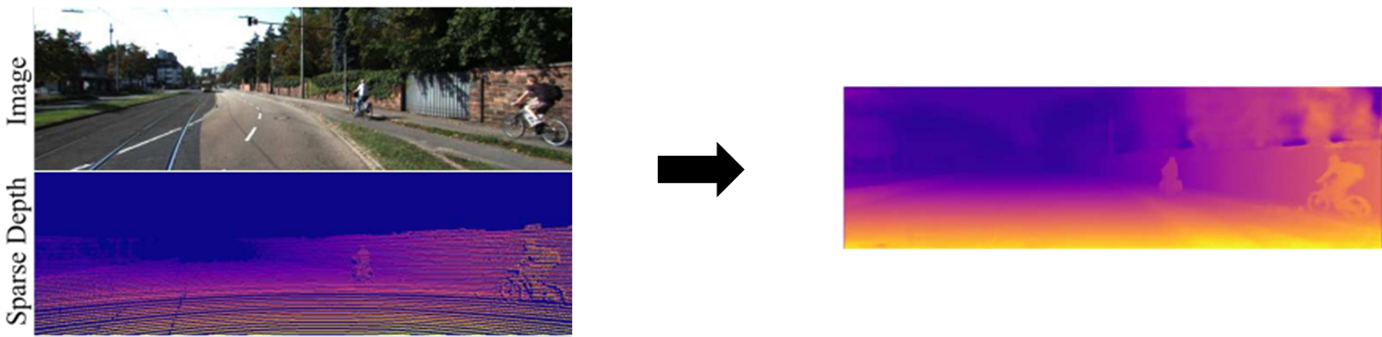
Fig. 1: The depth completion task.
Depth completion starts from a sparse set of known depth values and estimates the unknown depths for the remaining image pixels.
Challenges
-
Recovering depth discontinuities is difficult because pixels in boundary regions suffer from ambiguity as to whether they belong to the foreground depth or the background depth.
–> The paper proposes a multi-hypothesis depth representation that explicitly models both foreground and background depths in the difficult occlusion-boundary regions.
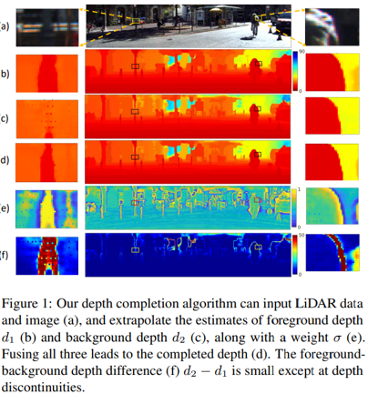
Fig. 2: Illustration of the proposed method.
Ambiguities in the Depth Completion Task
Ambiguities have a significant impact on depth completion, and it is useful to have a quantitative way to assess their impact. In this paper, the authors propose using the expected loss to predict and explain the impact of ambiguities on a trained network.
Simplifying Scene Assumption
The analysis makes a further simplifying assumption that there is at most a binary ambiguity per pixel. A binary ambiguity is described by a pixel having probabilities $p_1$ and $p_2$ of depths $d_1$ and $d_2$, respectively. When $d_1$ < $d_2$, we call $d_1$ the foreground depth and $d_2$ the background depth.
Modeling Ambiguities with the Expected Loss
To assess the impact of ambiguities on the network, we build a quantitative model. Consider a single pixel with a predicted depth $d$ and a set of ambiguities $d_i$, each with probability $p_i$; that is, each $d_i$ may act as the ground-truth depth with probability $p_i$. We then define the expected loss as a function of depth:
\[E\{L(d)\}=\sum_i p_i L(d-d_i)\]With the simplifying assumption above, this becomes:
\[E\{L(d)\}=p_1 L(d-d_1) + p_2 L(d-d_2)\]Note that the expected loss expresses the optimization objective of training; it is used to predict the behavior of a trained network at ambiguities and thus to justify the design of the proposed method. You may wonder how to determine $p_i$ — keep this question in mind; we will return to it later.
Designing the Loss Functions
The loss function is a key component of depth completion. The authors propose two asymmetric loss functions to learn the foreground and background depths, and a fusion loss to learn how to select or blend between them.
Foreground and Background Estimators
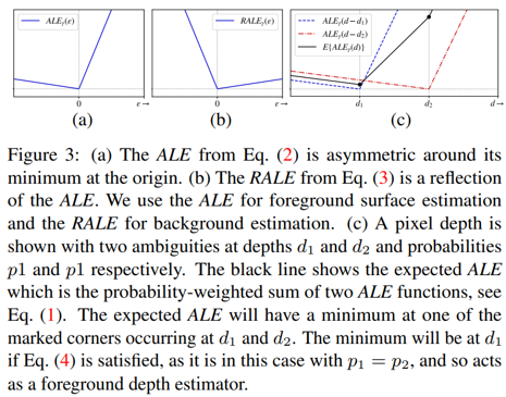
Fig. 3: The Asymmetric Linear Error (ALE) and its twin.
In this paper, the authors use a pair of error functions, as shown in Fig. 3, called the Asymmetric Linear Error ($ALE$) and its twin, the Reflected Asymmetric Linear Error ($RALE$), defined as:
\[ALE_{\gamma}=max(-\frac{1}{\gamma} \varepsilon, \gamma \varepsilon)\] \[RALE_{\gamma}=max(\frac{1}{\gamma} \varepsilon, -\gamma \varepsilon)\]Here $\varepsilon$ is the difference between the measurement and the ground truth, $\gamma$ is a parameter, and $max(𝑎,𝑏)$ returns the larger of $𝑎$ and $𝑏$. Note that if $\gamma$ is replaced by $1/\gamma$, both the $ALE$ and $RALE$ are reflected. Thus, without loss of generality, we restrict $\gamma \geq 1$ in this work.
To estimate the foreground depth, the authors propose minimizing the mean $ALE$ over all pixels to obtain $\hat{d}_1$, the estimated foreground surface. By examining the expected $ALE$, we can see what an ideal network will predict.
The full expected $ALE$ loss will be:
\[E\{L(d)\}=E\{ALE_{\gamma}(\varepsilon)\}\] \[=p_1 ALE_{\gamma}(d-d_1) + p_2 ALE_{\gamma}(d-d_2)\] \[=p_1 max(-\frac{1}{\gamma} (d-d_1), \gamma (d-d_1)) + p_2 max(-\frac{1}{\gamma} (d-d_2), \gamma (d-d_2))\]We obtain the expected losses at the ambiguities $d_1$ and $d_2$:
\[E\{L(d_1)\}=p_1 max(-\frac{1}{\gamma} (d_1-d_1), \gamma (d_1-d_1)) + p_2 max(-\frac{1}{\gamma} (d_1-d_2), \gamma (d_1-d_2))\] \[=p_2 (-\frac{1}{\gamma} (-(d_2-d_1))), \because d_1 < d_2\] \[=p_2 \frac{1}{\gamma} (d_2-d_1)\] \[E\{L(d_2)\}=p_1 max(-\frac{1}{\gamma} (d_2-d_1), \gamma (d_2-d_1)) + p_2 max(-\frac{1}{\gamma} (d_2-d_2), \gamma (d_2-d_2))\] \[=p_1 \gamma (d_2-d_1), \because d_1 < d_2\]For the estimator to prefer the foreground depth, the following must hold:
\[L(d_1)<L(d_2)\]This inequality is satisfied only when:
\[p_2 \frac{1}{\gamma} (d_2-d_1) < p_1 \gamma (d_2-d_1)\] \[\gamma > \sqrt{\frac{p_2}{p_1}} \qquad (Constraint \; 1)\]Fig. 4 demonstrates the behavior of the foreground depth estimator. We fix $d_1$ and $d_2$ to $4$ and $8$, respectively, and dynamically change the ratio of $p_1$ to $p_2$ to show that a properly restricted $\gamma$ is needed.
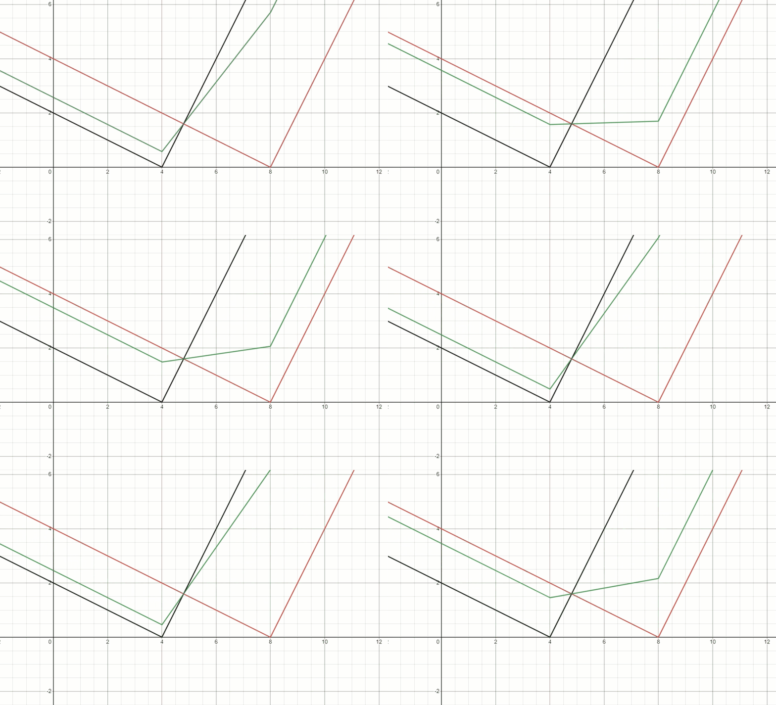
Fig. 4: The behavior of the foreground depth estimator.
By the same analysis, to estimate the background depth, the authors propose minimizing the mean $RALE$ over all pixels to obtain $\hat{d}_2$, the estimated background surface. Examining the expected $RALE$ yields the same constraint on $\gamma$, except that the probability ratio is inverted.
The full expected $RALE$ loss will be:
\[E\{L(d)\}=E\{RALE_{\gamma}(\varepsilon)\}\] \[=p_1 RALE_{\gamma}(d-d_1) + p_2 RALE_{\gamma}(d-d_2)\] \[=p_1 max(\frac{1}{\gamma} (d-d_1), -\gamma (d-d_1)) + p_2 max(\frac{1}{\gamma} (d-d_2), -\gamma (d-d_2))\]We obtain the expected losses at the ambiguities $d_1$ and $d_2$:
\[E\{L(d_1)\}=p_1 max(\frac{1}{\gamma} (d_1-d_1), -\gamma (d_1-d_1)) + p_2 max(\frac{1}{\gamma} (d_1-d_2), -\gamma (d_1-d_2))\] \[=p_2 \gamma (d_2-d_1), \because d_1 < d_2\] \[E\{L(d_2)\}=p_1 max(\frac{1}{\gamma} (d_2-d_1), -\gamma (d_2-d_1)) + p_2 max(\frac{1}{\gamma} (d_2-d_2), -\gamma (d_2-d_2))\] \[=p_1 \frac{1}{\gamma} (d_2-d_1), \because d_1 < d_2\]For the estimator to prefer the background depth, the following must hold:
\[L(d_1)>L(d_2)\]This inequality is satisfied only when:
\[p_2 \gamma (d_2-d_1) > p_1 \frac{1}{\gamma} (d_2-d_1)\] \[\gamma > \sqrt{\frac{p_1}{p_2}} \qquad (Constraint \; 2)\]Fused Depth Estimator
We desire a fused depth predictor, knowing that the foreground and background depth estimates provide lower and upper bounds on the depth of each pixel. We express the final fused depth estimate $\hat{d}_t$ for the true depth $d_t$ as a weighted combination of the two depths:
\[\hat{d}_t = \sigma \hat{d}_1 + (1-\sigma) \hat{d}_2\]where $\sigma$ is an estimated value between $0$ and $1$. We use a mean absolute error as part of the fusion loss:
\[F(\sigma)=|\hat{d}_t-d_t|=|\sigma \hat{d}_1 + (1-\sigma) \hat{d}_2-d_t|\]To analyze the fused depth estimate, we examine the loss below:
\[L(\sigma) = E\{F(\sigma)\} = p|\sigma \hat{d}_1 + (1-\sigma) \hat{d}_2-d_1| + (1-p)|\sigma \hat{d}_1 + (1-\sigma) \hat{d}_2-d_2|\]Here, $p=p_1$ and $p_2=1-p$. This has a minimum at $\sigma=1$ when $𝑝>0.5$ and a minimum at $\sigma=0$ when $𝑝<0.5$. We also draw the loss surface of $L(\sigma)$ in Fig. 5; the optimization direction guides the model to predict either the foreground depth $d_1$ or the background depth $d_2$.
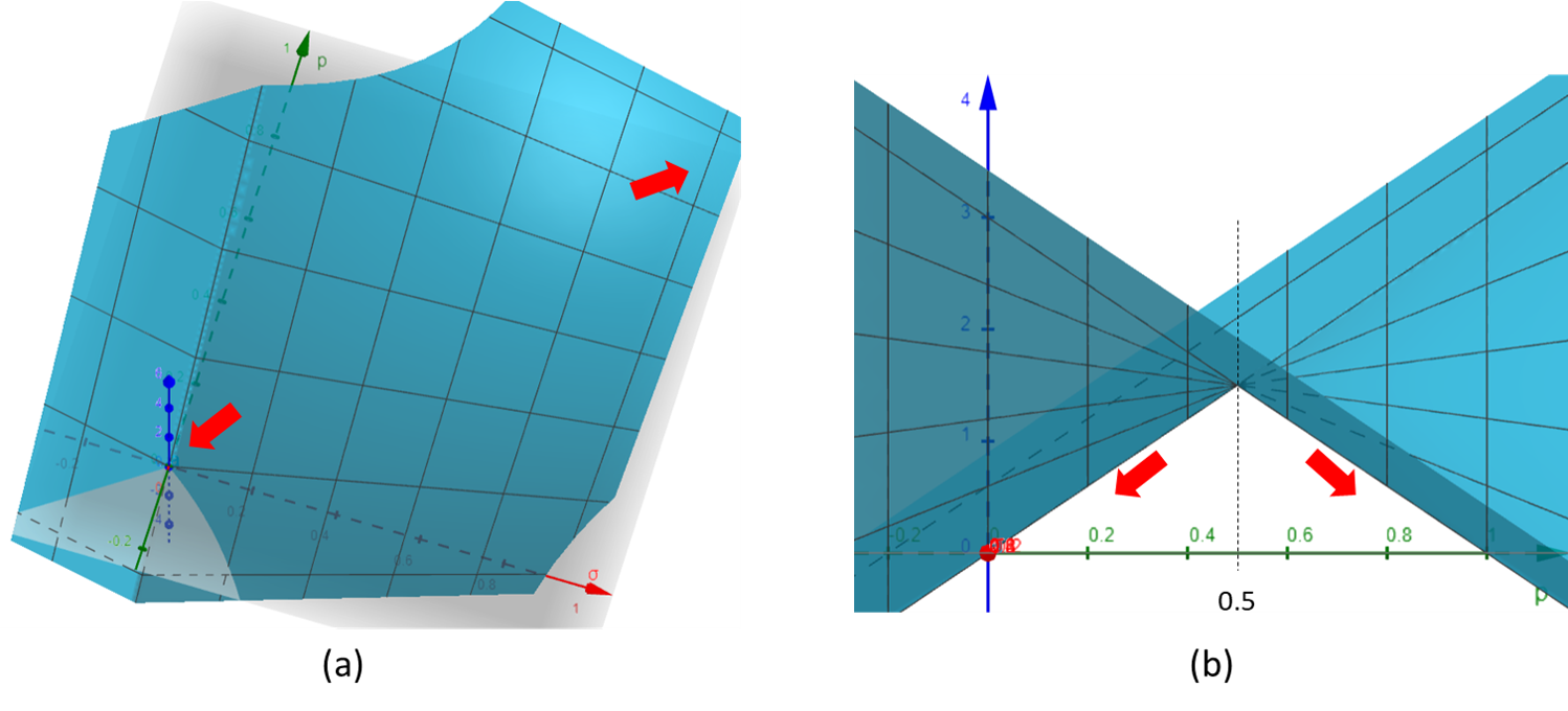
Fig. 5: The loss surface of $L(\sigma)$.
Depth Representation
We have developed three separate loss functions whose individual optimizations give us three separate components of the final depth estimate for each pixel. Based on the characterization of these losses, we require the network to produce a three-channel output. For simplicity, we combine all loss functions into a single loss:
\[L(c_1, c_2, c_3) = \frac{1}{N} \sum_{j}^{N}(ALE_{\gamma}(c_{1j}-d_1) + RALE_{\gamma}(c_{2j}-d_2) + F(s(c_{3j})))\]Here $𝑐_{𝑖𝑗}$ refers to pixel $j$ of channel $i$, $s()$ is the sigmoid function, and the mean is taken over all $𝑁$ pixels. We interpret the outputs of these three channels for a trained network as
\[𝑐_1 \rightarrow \hat{d}_1, 𝑐_2 \rightarrow \hat{d}_2, s(𝑐_3) \rightarrow \sigma\]Now let us see what happens when we force $p_1$ to be $1$ and $p_2$ to be $0$, which means the model learns to predict the depth $d$ considering only the foreground depth $d_1$ as the ground-truth depth $d_t$. Given $p_1=1$, $p_2=0$, and $d=\hat{d}_1$:
\[E\{ALE_{\gamma}(\varepsilon)\}=p_1 ALE_{\gamma}(d-d_1) + p_2 ALE_{\gamma}(d-d_2)\] \[=ALE_{\gamma}(\hat{d}_1-d_1)\]By the same token, we have:
\[E\{RALE_{\gamma}(\varepsilon)\}=p_1 RALE_{\gamma}(d-d_1) + p_2 RALE_{\gamma}(d-d_2)\] \[=RALE_{\gamma}(\hat{d}_2-d_2)\]We can further interpret this as follows: when a pixel is located at the boundary between foreground and background, $ALE$ tends to guide the model to predict $\hat{d}_1$ as the foreground depth $d_1$, while $RALE$ tends to guide the model to predict $\hat{d}_2$ as the background depth $d_2$. See Fig. 6:
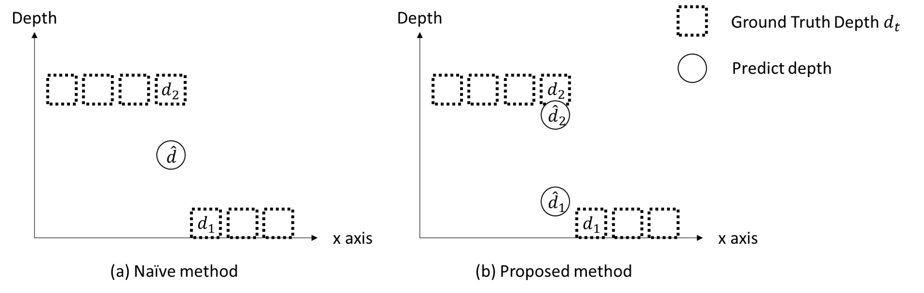
Fig. 6: Visualization of the model behavior.
Finally, we have:
\[L(c_1, c_2, c_3) = \frac{1}{N} \sum_{j}^{N}(ALE_{\gamma}(c_{1j}-d_t) + RALE_{\gamma}(c_{2j}-d_t) + F(s(c_{3j})))\]Note that, by doing so, Constraints 1 and 2 mentioned above are also satisfied.
Results
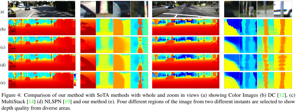
Fig. 7: Comparison of the proposed method with the state of the art.
Conclusions
- This paper proposes a twin-surface representation that estimates the foreground, background, and fused depths.
- This paper adopts a pair of asymmetric loss functions to explicitly predict foreground and background object surfaces.
References
[1] Saif Imran, Xiaoming Liu, and Daniel Morris. Depth completion with twin surface extrapolation at occlusion boundaries. In CVPR, pages 2583–2592, 2021.